Gesture Signal Processing
Offsets and Scaling
Often it is the case that we have a sensor input s in the range [a b] representing some gesturemade by the musician, but for the purposes of sound synthesis, we would like to transform the input to the target range [c d]. For example, we might have a=0, b=255, c=100, and d=500 if we wanted to use an 8-bit analog input to control an oscillator's frequency over the range 100Hz to 500Hz. We could implement the mapping on the AVR itself before sending the data over OSC, but it is usually easier to implement the mapping in Pd.
One way to map the sensor input to the target range [c d] is to apply an affine transformation. Below we have a signal flow diagram that shows how to process the input signal to derive a control signal ranging over the target range.
The diagram explains that we must made the following steps:
1) subtract out the input offset
2) scale the width of the range
3) add in the output offset
Mathematically, we have that the output z = (s-a)*(d-c)/(b-a) + c.
More complicated nonlinear mappings can sometimes be useful. For example, from a psychoacoustic perspective, it is better to create a logarithmic relationship between the position of a slider and the volume of a sound than to use an affine mapping. See Hans-Christoph Steiner's work on implementing some other nonlinear mappings in Pd.
Filtering
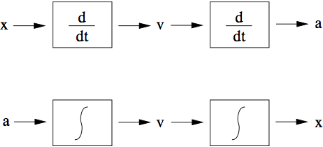
While studying sensors, we discovered that often a particular sensor will measure the position x, velocity v, or acceleration a of an object. However, we might like to use a different variable to control the way we synthesize sound. Ideally, integration and differentiation can be applied to convert between variables.
Filter Approximating An Integrator
In this case, we integrate an acceleration measurement in order to obtain velocity. We see that with each time step, v is updated to be nearly the same as the previous v, but it is affected by the input a. This is an example of a low-pass filter because the filter passes mainly low frequencies.
v = 0.1*a + 0.9*v;
Filter Approximating A Differentiator
Next we show how to approximate a differentiator, so now x represents a measured position, and v represents velocity. The extra variable r is introduced to represent the previous position measurement. T is the sampling interval, or the time in seconds between samples. Hence, the estimated velocity is the scaled difference between the current position and the previous position. This filter is an example of a high-pass filter because it passes mainly high frequencies.
v = T*(x - r);
r = x;
Filter design is an important part of the field of signal processing. For more details, see Julius Smith's book on basic filter design.
Thresholding
Often we want to implement some sort of event detector. For instance, we may want to detect the event that the musician has struck an object such as a drum. If the musician is holding an accelerometer in his or her hand, we can detect the event by waiting for a large value or a large change in the accelerometer signal.
For more details on thresholding, see the threshold and threshold~ objects' help patches in Pd.
Interpolation
Interpolation is a method of constructing new data points within the range of a discrete set of known data points.
Interpolation In Time
We have already learned about using the line~ object in Pd to interpolate in time to avoid zipper noise.
Interpolation In Space
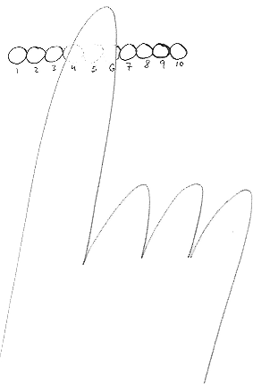
Now we consider interpolation in space. Given a finite number of sensors at discrete positions, we might want to estimate the continuous position of an object in space. For example, imagine a line of 10 force sensing resistors or capacitative sensors as shown below.
We can develop an estimate of the center of the user's finger using linear interpolation. Let's say that the centers of the 4th, 5th, and 6th sensors are located at the horizontal positions 20mm, 25mm, and 30mm, respectively. If s4, s5, and s6 represent the sensor inputs from the 4th, 5th, and 6th sensors, respectively, then the following expression estimates the continuous position of the center of the finger:
(20mm)*s4 + (25mm)*s5 + (30mm)*s6
--------------------------------------------------------
s4 + s5 + s6
Note that for this technique to work well, the sensors should be well matched. The expression also should not be evaluated if s4 + s5 + s6 is small, in which case the user is not pressing hard enough on the array of sensors.
Written by Edgar Berdahl, 10/08


